Vlookup and Trial Balances Function and Example
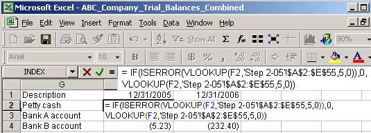
That happens because VLOOKUP cannot find accounts 8022 and 8023 in the 12/31/05 trial balance file. Remember that those accounts were not used during 2005 and were introduced in 2006. We would like to get rid of those "#N/A" because they will not let us create totals. We can do that by altering our VLOOKUP function to read as follows:
= IF(ISERROR(VLOOKUP(F2,'Step 2-05'!$A$2:$E$55,5,0)),0,VLOOKUP(F2,'Step 2-05'!$A$2:$E$55,5,0))
The formula seems to be complicated, but it just looks so. Let's brake it into pieces. We will name VLOOKUP(F2,'Step 2-05'!$A$2:$E$55,5,0) as VLOOKUP for simplicity. So we have:
= IF ( ISERROR(VLOOKUP), 0, VLOOKUP )
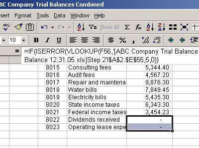
Function ISERROR checks whatever it is between the parenthesis to see if that gives an error. If it does, this function returns TRUE and if it does not, it returns FALSE. Thus, we can read the above formula as follows: If VLOOKUP cannot find an account in 12/31/05 trial balance (and returns an error), then ISERROR returns TRUE and IF function results a zero. On the other hand, if VLOOKUP can find an account in 12/31/05 trial balance (and does not return an error), then ISERROR returns FLASE and IF function returns the value provided by VLOOKUP function:

Once we copy the above formula to the bottom, we can see that rows 56 and 57 have zeros instead of "#N/A". That is exactly what we were trying to accomplish:

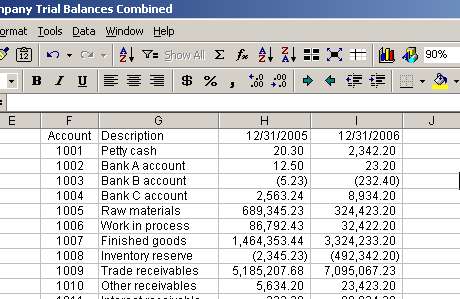
We use a similar approach to pull in data from 12/31/06 balances. The same formula (with IF, ISERROR and VLOOKUP) can be used with a minor modification to the second argument:
=IF(ISERROR(VLOOKUP(F2,'Step 2-06'!$A$2:$E$54,5,0)),0, VLOOKUP(F2,'Step 2-06'!$A$2:$E$54,5,0))

Page 6 of 7