Vlookup Function, Vlookup Syntax, Vlookup Examples
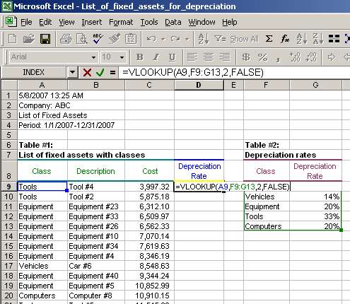
Of course, we could sort the entire fixed assets list by the fixed asset class and manually enter depreciation rates. However, why do that if we can use vlookup and finish this task in less than a minute without additional hassle? Let us see how to use vlookup in this situation.
First, we need to identify the arguments for VLOOKUP:
- lookup_value - as mentioned before, this is the value by which we can link two tables together. In our case, the linking field is the fixed asset class because both tables have it. So, the values in column A will be our lookup_values.
- table_array - this is the source from where we will be pulling the depreciation rates. In our case, Table #2 is where such depreciation rates are stored, so the table_array is cells F9-G13.
- col_index_num - this is the number of the column, starting from the very first column with the linking field (fixed asset class), in which our depreciation rates are stored. There are two columns in Table #2. The first one is Class and the second one is Depreciation Rates. We need depreciation rates column; thus, the col_index_num is two (2).
- range_lookup - we want to find exact matches of depreciation rates for our fixed assets. So, we will use FALSE for this argument.
Second, we enter the formula using the identified arguments in cell D9:
=VLOOKUP(A9,F9:G13,2,FALSE), where
- A9 is lookup_value
- F9:G13 is table_array;
- 2 is col_index_num; and
- FALSE is range_lookup.

Note that the result is 33% in cell D9. VLOOKUP correctly identified that the fixed asset class for Tool #4 is Tools. Then it found the same class in Table #2, took the 33% depreciation rate from the second column in Table #2 and returned this 33% value in cell D9.
Page 2 of 3