Sumif Function, Sumif Syntax, Sumif Examples
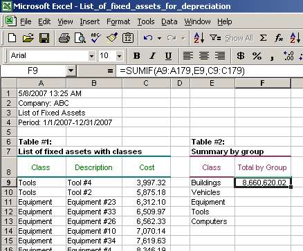
Of course, we could sort the entire fixed assets list by class and summarize fixed asset costs for each class. However, why do that if we can use SUMIF and finish this task in 1 minute without additional hassle? Let's see how to use SUMIF in this situation.
First, we need to identify the arguments to SUMIF:
- range - as mentioned before, this is a range of cells that we want to evaluate for a criteria (see below for the criteria). In our case, the range is cells within Table #1 with classes, or A9-A179. These cells include class identifiers for all fixed assets in Table #1;
- criteria - as we would like to summarize fixed assets by class, criteria is a unique fixed asset class. For example, the criteria may be "Buildings," "Vehicles," and others from cells F9-F13 in Table #2;
- sum_range are the actual cells to sum. We want to have totals for fixed asset costs. Such costs are shown in Table #1, cells C9-C179. Thus, the sum_range is cells C9-C179.
Second, we enter the formula using above identified arguments in cell F9 for the first criteria ("Buildings"):
=SUMIF(A9:A179,E9,C9:C179), where
- A9:A179 is range;
- E9 is criteria;
- C9:C179 is sum_range.

Note that the result is 8,660,620.02 in cell F9. SUMIF summarized costs of all fixed assets with class Buildings. In other words, 8,660,620.02 is the total of costs in column C with fixed asset class in column A equal to "Building."
Third, we need to ensure that our range and sum_range do not shift when we copy the formula down in column F. So, we need to change range and sum_range cell references from relative to absolute by adding the dollar sign ("$") before them as shown below:
=SUMIF ( $A$9:$A$179, E9, $C$9:$C$179 )
In case we do not change the cell references from relative to absolute, the range and sum_range will shift when the SUMIF formula is copied from cell F9 to cells below and cause an incorrect result. At the same time, note that the criteria cell reference should remain relative as we want it to change (from E9 to E10 to E11 to E12 to E13) as we copy the formula down.
Page 2 of 3